
GLM-5.2 RL weight transfer in 4 seconds using NIXL and ModelExpress

GLM-5.2 RL weight transfer in 4 seconds using NIXL and ModelExpress
In RL at 1T Scale, we detailed how prime-rl trains trillion-parameter models like GLM-5 with sub-5-minute step times on just 28 H200 nodes. That speedup exposed a new bottleneck: syncing updated weights from trainer to inference after every step, which stayed stuck at 60-90 seconds no matter how fast everything else got. Here, we rebuild that hand-off on NIXL and ModelExpress, cutting weight transfer for GLM-5.2 down to single-digit seconds and removing the static-process-group constraints that stood in the way of fault-tolerant, elastic inference.
Weight transfer in RL
The models being trained grow larger and larger every day. To serve these models efficiently, we require more compute and more memory. Post-training introduces another bottleneck—weight transfer—when post-training, after every optimizer step, the policy needs to be synchronized from the trainer to the sampler. This requires transferring the model weights (or their change in time) between a set of workers. These payloads grow to sizes of multiple terabytes. Common solutions, such as using NCCL for intra-datacenter updates, or file-system, potentially delta-based updates for inter-datacenter updates have their drawbacks and tradeoffs.

g_i and inference policy versions θ_i on concurrent timelines.There are various approaches to weight transfer. Most RL frameworks, including prime-rl, implement a subset of them. We’ll cover the most common approaches, their drawbacks, and how we decided to solve them with NIXL.
Weight transfer in prime-rl
Let’s start with the most common approach - NCCL. NCCL-based transfer requires a static process group - this fact makes fault-tolerance or elasticity difficult, almost impossible, at scale. On top of that, NCCL with sharding-aware P2P transfer introduces common synchronization points and often doesn’t fully utilize the network bandwidth. However, if your workload doesn’t require either of those, NCCL is often the best choice that is easy to implement and provides decent performance. File-system, potentially delta-based updates utilize a shared filesystem, often on network, such as S3 - to upload either a full copy of new weights, or a delta from the last step. As (remote) filesystem upload is often-times slow, this type of implementation is usable for smaller models, respectively when the inference engine enables delta-based reloads in a scalable way. Common use-cases for this are cross-datacenter workloads. For our workloads, NCCL was becoming slower and slower and its static process group was becoming an obstacle in our work towards fault-tolerant and auto-scalable inference. That’s why we’ve decided to use remote direct memory access (RDMA) based weight transfers to solve this. This required us to solve an interesting problem that arrises from being model agnostic (weight format), which we’ll talk about below. However, first we have to start with RDMA and how we can harness its power.
RDMA and NIXL primer
As an honest note - this work was heavily inspired by the work of Lequn Chen in Journey to 2-second Inter-node RL Weight Transfer, while adding some magic on top, to handle some vLLM ↔ prime-rl quirks.
I won’t go into detail on how remote direct memory access (RDMA) works. For the sake of this post, it’s only necessary to think about RDMA as a way to directly access remote memory - a GPU on a remote node in our case. This allows us to bypass synchronization and transfer directly over a source and destination network interface cards (NICs).
We will also focus only on one-sided RDMA, which bypasses CPU, resulting in lower latency. RDMA can be split into 2 “paradigms” - PUSH and PULL. The names are fairly self-explanatory: PUSH writes local data to a remote memory segment, PULL pulls remote data and writes them to a local memory segment.
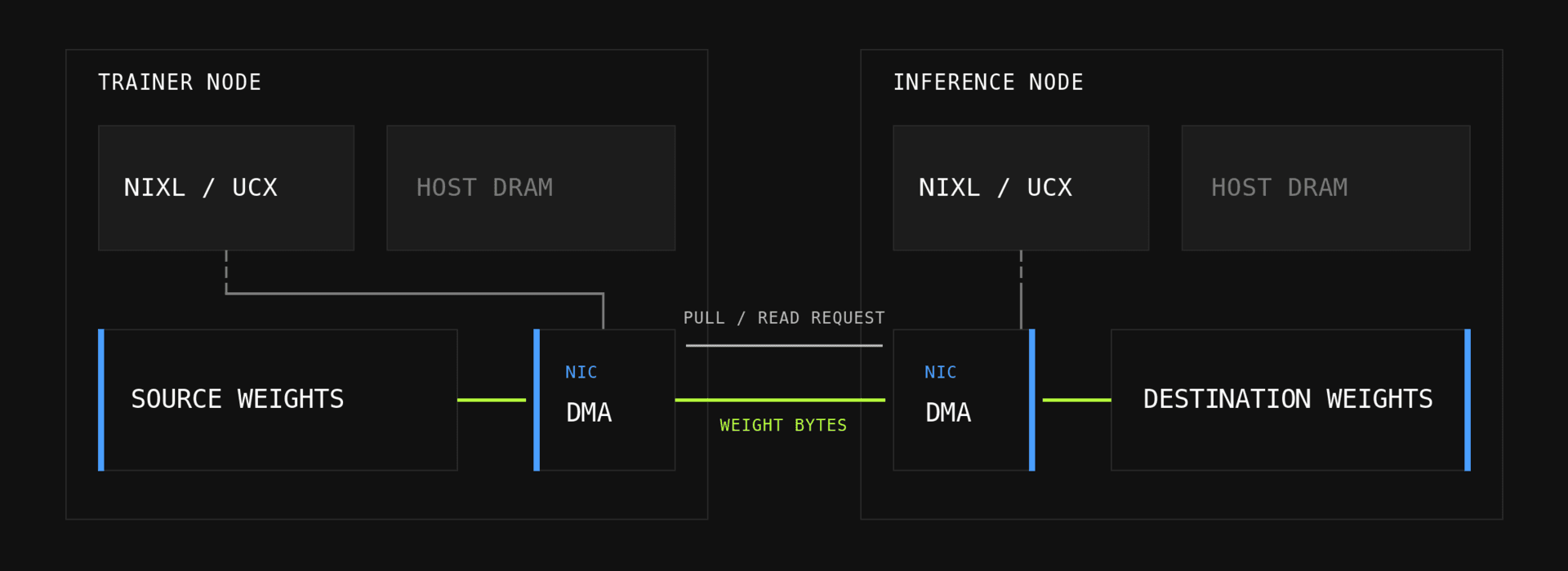
Hardware support
Most of the current data-center grade machines come equipped with a single 400Gb/s NIC per GPU (800Gb/s if ConnectX-8 SuperNIC is used - for example in (G)B300 clusters). We can directly utilize this network and RDMA to read and write from/to remote memory across the cluster.
These abstractions are already implemented in various open-source libraries, which we’ll use in this work, mainly https://github.com/ai-dynamo/nixl from nvidia-dynamo team, that builds on top of https://github.com/openucx/ucx - Unified Communication X: a library that abstracts the transfer-level primitives, allowing NIXL to be somewhat transfer level agnostic. This also lets us to not worry about things as rkey, lkey and memory consistency models.
Sky is the limit
To start with our implementation, we need to know what’s the best we can get. If we do some boring math, we can derive a lower bound that even perfect code cannot beat. Let be the total bf16 weight payload and the usable bandwidth of one GPU’s NIC. For our example, we’ll use GLM 5.2 in bf16 giving us . Assuming a trainer FSDP world size of and an inference data and expert-parallel world size of , with the weights distributed evenly across ranks (we can safely assume that experts are majority of the storage, and that the rest is negligible).
Each trainer rank and therefore each trainer NIC must send , while each inference rank/NIC must receive . Plugging in the payload size:
This means that there will be more data flowing through inference NICS, so the lower bound is as follows:
Plugging in the NIC parameters from section Hardware support:
This leaves us with a theoretical ceiling of 1.0 sec
Sky might not be the limit
Is it really this simple - just take a local and remote pointer, ask the NIC to move the bytes and be done with it? Not quite, if it was you wouldn’t be reading this blog. The remaining problem is that the trainer and sampler (in our case vLLM) do not necessarily store the same logical weight in the same physical layout. This is particularly important for our NIXL based approach - we can ask the NIC to move bytes, but how do we know what is the mapping between the trainer and inference bytes. What if there is some processing happening? We will cover our approach to this in the following sections.
Weight format hell
vLLM starts from checkpoint-format tensors - the names, shapes, and dtypes stored on disk or the Hugging Face Hub - and transforms them into runtime kernel format. The result depends on the model architecture, parallelism strategy, GPU, quantization mode, and selected kernels.
For example, an MoE loader may pack the gate and up projections (w1 and w3) into w13_weight. Quantized kernels may additionally cast, transpose, pack, or swizzle weights and scales into backend-specific layouts such as those consumed by tcgen05. Other kernels might pack the gate and up projections (w1 and w3) into w31_weight - there are no limits to what the runtime format is.
A trainer parameter therefore does not map to one obvious inference address. Hard-coding this mapping would duplicate vLLM’s loader for every model, kernel, and configuration. Performing all transformations on the trainer would also require inference-aware sharding and enough temporary memory for another model-sized representation.
However we can do better - with some clever PyTorch magic, we can “record” all the operations executed on an underlying storage, and store them in a form of a graph.
This graph can then be naturally split at the first view that materializes new storage - this can for example be a cast to another datatype.
Every operation before this point is a storage-preserving view - this can be represented as an operation that transforms the stride and offset of the base storage, and together with the base pointer allows for a view into the remote storage with a transformed stride and offset.
Past the aforementioned splitting point, we’re left with operations that operate on the data, not just offsets and strides. This suffix is then replayed on the inference GPUs on the transfered data that were a result of the prefix.
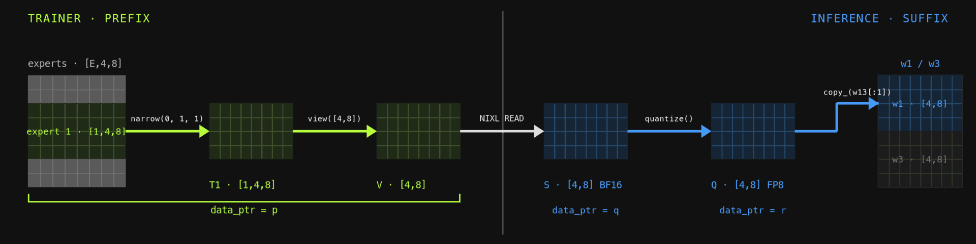
data_ptr, updated offset, shape, and stride. Suffix: materializing operations replayed on inference before writing w13_weight.Discovering vLLM’s runtime layout
The tracing approach is inspired by vLLM’s Ray Direct Transport proof of concept, which uses a tensor subclass to discover how a running model expects its weights to be loaded.
Prime-rl adds another layout boundary: the trainer checkpoint uses prime-rl names and layouts rather than a one-to-one copy of the Hugging Face checkpoint. During initialization, we create one LazyWeight for every tensor described by the TrainerTensorTable. Each wrapper carries the source name, shape, wire dtype, device, and recorder, but owns no weight payload.
We first run the normal prime-rl-to-HF conversion chain over this lazy state. The resulting HF-named values are then passed through vLLM’s real load_weights path. LazyWeight.__torch_function__ intercepts supported operations such as view, narrow, split, permute, contiguous, and dtype casts, appending each one to an operation chain. Equivalent operations on meta tensors propagate the resulting shape, stride, and dtype without touching live model storage.
When the loader reaches its terminal copy_, we record a RecordedCopy: the original trainer source, the complete operation chain, and the exact destination module, tensor name, offset, shape, and stride. This connects a logical trainer weight to the actual vLLM kernel storage without a handwritten mapping for every model and kernel.
For each recorded copy, plan_tensor_replay finds the longest storage-preserving prefix. The resulting TensorReplayPlan contains the source offset, shape, and stride, which can then be used to access the remote storage, plus the materializing or dtype-changing suffix that must be replayed locally. The routing layer then maps that source view across the trainer’s FSDP shards.
Tracing and planning happen once. On every weight update, inference reuses the plan: NIXL pulls the routed source bytes into GPU memory, the replay suffix runs on the inference GPU, and a final copy_ updates the live kernel tensor.
A tensor’s journey: from trainer storage to live vLLM weights
Let’s follow one representative expert tensor through the system. The exact names and operations vary by model and kernel, but the lifecycle is the same.
1. Trainer tensor identity
In the FSDP layout used here, a logical tensor is sharded along dimension 0. A trainer rank may own only a flat interval of its rows. The TrainerTensorTable records the information needed to address those shards:
- global tensor name and shape;
- wire dtype: BF16 by default, or FP32 when the model marks the tensor with
keep_in_fp32_for_weight_transfer; - transfer group;
- owning NIXL agent, logical offset, element count, and registered GPU address.
ModelExpress publishes this table during initialization.
2. Inference records the loader path
Inference creates a lazy tensor with the trainer source name, shape, and wire dtype. It runs that tensor through the normal Prime-to-Hugging Face conversion and vLLM’s real load_weights path.
LazyWeight.__torch_function__ records operations such as view, narrow, split, permute, contiguous, and dtype casts. When the loader reaches its terminal copy_, the trace contains the trainer source, the full operation chain, and the exact destination tensor, offset, shape, and stride.
3. Split addressing from replay
plan_tensor_replay splits the chain at the first operation that changes dtype or allocates new storage.
| Recorded step | Memory effect | Transfer plan |
|---|---|---|
select, narrow, or a view-producing transpose/permute | Still references the source allocation | Compile into source offset, shape, and stride |
contiguous, a dtype cast, quantization, or another materializing operation | Creates new storage or representation | Replay on the inference GPU |
Terminal copy_ | Writes the live kernel parameter | Record the exact destination view |
The prefix becomes source addressing. Only the materializing suffix runs after transfer.
4. Route across trainer shards
The source view may span multiple trainer ranks. Routing intersects that view with FSDP ownership and creates the reads needed to fill the inference staging tensor. Each route contains:
- trainer agent;
- source address;
- destination address;
- byte count.
NIXL executes these as direct GPU-memory reads. Multiple trainer shards can write into disjoint ranges of the same inference staging tensor.
5. Replay and load
Once the reads complete, each inference rank:
- reconstructs the recorded source view over staging memory;
- runs the materializing suffix, including online quantization when required;
- copies the result into the recorded vLLM destination view;
- runs the layer’s remaining post-load processing.
6. Overlap transfer and replay
With weight_broadcast.overlap_transfer_and_replay = true, inference can replay and quantize group N while NIXL transfers group N+1. This needs at least two staging buffers, but hides most of the online quantization time.
In this example, trainer GPU0 owns one contiguous [E=2, M=4, N=8] tensor containing experts 7 and 8. Inference ranks 0 and 1 each narrow to one expert, issue separate NIXL READs into BF16 staging tensors, replay FP8 quantization, and copy the FP8 weights into their local vLLM tensors; quantization emits the scale tensors separately. See the lifecycle overview below for the initialization and per-update sequence.
Lifecycle overview
| Once, during initialization | For every policy update |
|---|---|
| Publish the trainer tensor table and peer metadata through ModelExpress | Trainer stages each group and sends a versioned NIXL ready notification |
| Trace the real conversion and vLLM loader | Inference reposts prepared NIXL READs to every serving trainer rank |
| Split chains and compute shard routes | Inference replays and potentially online-quantizes group N while receiving group N+1 |
| Allocate/register staging arenas and prepare reusable READ descriptors | READ completion returns the trainer-arena credit |
End-to-end results
We measure time/broadcast_weights, which covers the full vLLM lifecycle: /pause → /update_weights → /resume. The setup uses 12 DGX H200 nodes, each with eight 400 Gbit/s Mellanox NICs. GLM-5.2 trains with FSDP=64 and EP=8 across eight nodes, then loads into DPEP=32 inference across four nodes. Inference applies fp8_per_block online quantization. We run 20 policy updates and report the median over equal 15-update windows for each path.
The NCCL baseline gathers each layer on rank 0 and broadcasts it, with a median of 86.1 seconds. Production NIXL with the existing sync/32 cadence reaches 9.3 seconds. Two effects account for most of the remaining gap to the initial one-second estimate:
- The measured receive volume per inference rank is roughly 2.2× the idealized 50 GB estimate because some operation chains materialize early and dense parameters do not follow the simple MoE sharding model. That raises the network floor to roughly 2.2 seconds.
/pausecan spend another 3–6 seconds waiting for distributed pause consensus.
During transfer, each NIC reaches roughly 45 GB/s of its 50 GB/s peak bandwidth. Most of the remaining latency comes from waiting for pause consensus.
/pause mechanism
With DPEP, vLLM executes request waves coordinated by DPCoordinator. A rank that receives /pause sets pending_pause = True, but it cannot stop immediately: other ranks may still enter EP collectives, and stopping one participant early would deadlock the group. The rank therefore keeps serving normal requests until every DP rank agrees that a pause is pending.
ParallelConfig.sync_dp_state establishes that agreement with an all-reduce. vLLM performs this consensus every 32 waves to avoid adding an all-reduce to every serving step.
In asynchronous reinforcement learning, the inference engine is always saturated, so it continues processing real requests during those 32 waves. The new policy cannot be applied until every rank reaches the next consensus point.
Let’s sync every step
We changed pause consensus from every 32 waves to every wave and reran the same benchmark. Median end-to-end time dropped to 3.9 seconds.
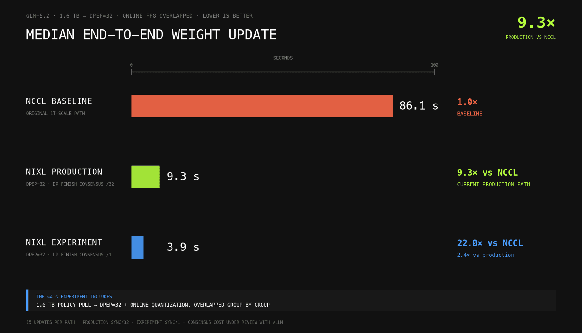
Those 3.9 seconds include transferring the full 1.6 TB policy into DPEP=32 inference and running online FP8 quantization. Transfer of the next group overlaps replay and quantization of the current group, so the quantization cost is largely hidden.
We are working with the vLLM team to measure whether sync/1 affects serving throughput and to make the cadence configurable.
Next steps
While the foundation is now in place, the biggest unlock of this work is not yet implemented. ModelExpress and NIXL don’t create a static process group - we want to follow-up on this work by implementing auto-scaling with blazingly fast inference start times. This closely ties to fault-tolerance across EP replicas (intra EP fault-tolerance is for another time) and liquid compute. If this is something that you enjoyed reading and would like to work on similar projects, let us know at Prime Intellect Jobs